In the functional world of the century-long flat Case-Shiller chart, families spent a stable portion of their incomes on rent and home prices reflected a stable premium on rents. Rents on existing homes remained flat, so that, as average incomes rose, existing homes filtered down to families with relatively lower incomes. New homes were built until the total rental value of homes increased to reflect the rise in incomes.
In a broad sense, in that functional world, I think it doesn’t matter much whether the growth is in real per capita income or in population. All you really need to know is real total income growth. If real GDP increases by 30% over a decade, you can expect the real value of the stock of housing to increase by 30%. It doesn’t matter if that consists of 10% population growth or 20%, or no population growth and 30% real per capita income growth.
The details about the houses will be different in those scenarios, but if you’re trying to forecast residential investment, aggregate rental expenditures, or aggregate real estate values, knowing that real total income growth will be 30% higher tells you almost everything you need to know.
This makes the residential real estate asset class different from equities. The growth of real estate can be thought of as a result of economic growth, whereas the corporate output that drives equity values creates economic growth. (That isn’t to say that housing isn’t productive or that innovations in housing construction can’t improve living standards.
It’s more of an accounting statement. Real housing, where legal, scales with income, and most of the increase in real incomes is associated with improvements in the 90% of economic growth outside of housing.)
Corporations also have rising and falling capacity utilization and the ability to increase capacity as the economy grows. So, a growing economy usually translates to higher profits and share prices for existing firms. But homes are fixed assets. When the economy grows, the total stock of real estate assets grows, but it grows through the addition or renovation of homes. Growth means that the existing homes claim a smaller share of the total rental value.
In other words, when the economy grows, there are some additional firms and innovations, but also, Microsoft (NASDAQ:MSFT) and Walmart (NYSE:WMT) will tend to grow with it. In a functional housing market, when the economy grows, your stock portfolio should grow, but your house should stay the same and become a smaller portion of the new stock of homes.
Or at least that’s how it should work. It’s how it worked for all those decades and centuries when the Case-Shiller chart was flat.
That means that the “beta” for individual homes is below 1. It isn’t zero. There are market imperfections, changing liquidity and credit access, etc. But, it’s very low.
The institutional real estate business tends to operate on stable rules of thumb. I remember years ago watching a presentation from a REIT, and they were talking about how their “cap rate” (the expected return on their investments before capital gains) had been 5 for years, but that their board had recently reduced it to 4.5 or something.
I took that at the time as a sign of a very under-developed market. In liquid, sophisticated markets, committees don’t set expected returns. Markets do. If you run a bond fund, you don’t decide what your returns are going to be. You look at the bids and asks at the Chicago Mercantile Exchange, and they tell you what your returns will be.
But, as I have settled into my “Upside down CAPM” way of thinking, I realized that this is simply a reflection of the stable expected returns that all at-risk investments earn. Equities have a stable expected return of 6%. It makes sense that real estate, with a low beta, has a slightly lower expected return, which would change slightly with real interest rates.
For years, long-term bond yields were typically around 4% and declined to 1%. If real estate trades as if it has a beta of 0.5, then its expected return would range from 3.5% to 5% over that period:
ERi = Rf + βi (ERm − Rf)
5% = 4% + 0.5 x (6% - 4%)
3.5% = 1% + 0.5 x (6% - 1%)
This has been a strange time with very low real interest rates. Negative real rates are unusual. So, a cap rate approximating 5% and appearing to be relatively fixed is pretty reasonable, and it would follow that committees in charge of REITs would consider adhering to that stable norm to be a part of the discipline of being active in that market.
The point here that I think might be interesting is that stable expected returns aren’t actually an oddity. Expected returns on all at-risk diversified portfolios are stable. Stable expected returns don’t make real estate different from equities. It makes them similar.
Note that this does mean that real estate valuations might be somewhat affected by interest rates. But it’s not because real estate is valued like bonds. It’s because real estate is like a low beta equity, so changes in the equity risk premium are muted and don’t fully revert to a stable expected return level.
I do think there may have been some broad increase in real estate values from the mid-1990s to the mid-2000s when real long-term bond yields declined from about 4% to 2% and the equity risk premium moved in the other direction. In the post-2008 period, as we have left the classic upside-down CAPM world with adequate new home construction, other factors have dominated changing home prices, and I have found that the weak association between interest rates and home values has been hard to find.
Real estate is like stocks and unlike bonds because expected returns are stable, and it’s like bonds and unlike stocks because experienced returns on a diversified portfolio of residential real estate are stable.
Of course, at first blush, that’s a crazy thing to say after 2008. However, 2008 was not a market equilibrium. It was a policy shock into disequilibrium.
Figure 1 shows the Zillow (NASDAQ:ZG) home price index for the United States from 2000 to June 2010. The Erdmann Housing Tracker attributes about 17.6% of home prices in December 2005 to cyclical price inflation and about 6.4% to the credit boom. A total of 24% overvaluation. Yet, even with a big recession, the average home price in the US would never have gone significantly negative if late 20th-century credit standards had been maintained.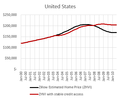
The old belief among homebuyers that supposedly caused the 2008 financial crisis that homes never lose value is basically true for a diversified portfolio of American homes. It was even true in 2008. We just chose to have a credit shock.
It’s true because in a functional market, real rents track real incomes and real incomes rarely decline enough to cause homes to lose substantial value.
Most cities during that period were something like Charlotte. Without the credit shock, home values would have continued rising moderately with inflation. In Figure 2, Charlotte home prices are shown rising in the absence of the credit shock, but that is because by 2008, supply conditions were poor everywhere. Construction had collapsed. We had already pushed virtually every city out of the functional market context.
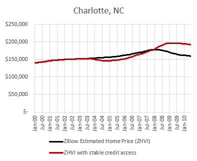
Home prices were simultaneously inflated by a supply shortage and deflated by a credit shock.
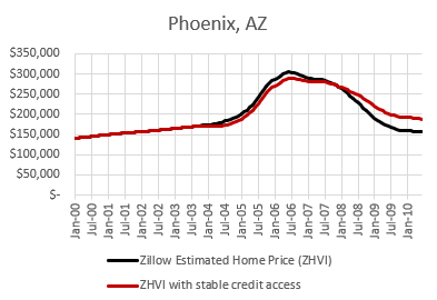
Phoenix was a city that likely had a correction coming in any case. Even after correcting for credit access, home values in Phoenix declined significantly after 2007. The Phoenix market got ahead of itself (much as Austin recently did). Local bubbles can happen.
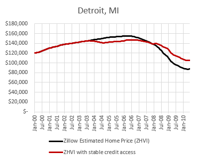
Detroit is another city where home prices would have fallen even with stable credit access, but not because of a bubble. In Detroit, prices declined even within the processes of a normal market. Detroit really suffered during that time, to the extent that there was substantial population decline.
From 2000 to 2010, total employment in Detroit dropped by 20%. Between 2003 and 2011, real rents in Detroit declined by 15%. In the classic Upside Down CAPM world, total incomes in Detroit suffered enough to lower the demand for housing below the supply of the existing stock of housing. Declining demand hit a vertical supply curve, and prices tumbled.
New York City had left the classic Upside Down CAPM world. By 2008, rents and prices in New York City were elevated because of a lack of new supply. Every residential structure was bundled with inflated land. And, even though land values were inflated, New York City home prices would have continued to rise moderately in the absence of a credit shock.
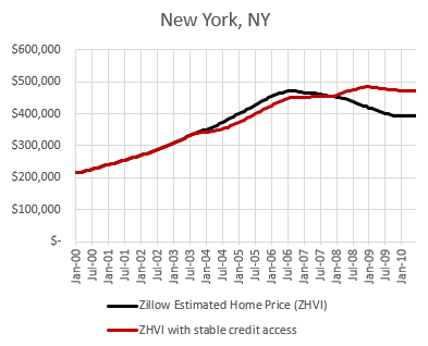
So we have the amply supplied Upside Down CAPM scenario, in which the only way that home prices will decline is through an economic downturn so steep that it reverses regional income growth. (Detroit in 2008).
And, there are two scenarios that diverge from an amply supplied Upside Down CAPM scenario. One scenario involves cyclically elevated home prices. Prices there are vulnerable to deflation. (Phoenix in 2008). One scenario involves secularly elevated home prices because of supply constraints, which lead to elevated land rents. (New York City in 2008). That scenario, to date, has been resistant to home price deflation.
Most cities today are in that scenario.
I will expand on that more in the next post.
