No one would characterize GDP forecasting as easy. Some might call it worthless. But to the extent that we crunch these numbers, it’s useful to note that there are many ways to slice and dice. Not surprisingly, results vary–sometimes by a lot. Among the various knives in this drawer is one with the potential to minimize the noise via modeling GDP changes on a year-over-year basis.
It’s flawed, of course, like every other effort at divining the future. But the underlying methodology has a certain appeal, as I’ll discuss. And maybe, just maybe, its flaws are less egregious vs. the usual suspects that attract so much attention in the GDP prediction game.
Let’s start with the focus on year-over-year changes. The logic is that annual trends reduce some of the noise. Quarterly changes, which dominate the discussion on all things GDP, are quite a bit more volatile and therefore harder to model. Does the use of year-over-year changes lead to a bit more reliability in forecasting? Maybe.
There are several ways to test this theory, including analyzing in-sample forecasts against the actual data and running various tests–root mean square error, for instance—to judge how the predictions hold up. That’s a worthwhile effort, but even better is tracking how the out-of-sample forecasts fare. But that takes time. Let’s start by projecting annual GDP growth for Q2. The official Q2 report, by which we’ll judge the forecast, is due for release on July 29.
To assist in keeping the noise that infects all forecasting to a minimum, let’s add another feature: multiple forecasts. There’s a large body of literature that demonstrates the superiority of combining forecasts, which tends to outperform any one forecast. To the extent that we tap into this feature in modeling, we’re probably boosting the odds for success—or reducing the odds for failure, if you prefer–if only modestly so.
For a real-world example, see my near-term estimates for the Economic Trend Index (ETI)—a proprietary benchmark I use for tracking the US business cycle. Each month, I publish ETI forecasts that gaze into the future. The results are encouraging, probably because of the nature of the forecasts—i.e., combining forecasts. The fact that I’m only looking ahead a few months helps, too, since the further out in time we look, the greater the potential for error.
ETI is a multi-factor benchmark and the forecasts are based on predicting each indicator, separately, and then aggregating the results to arrive at an ETI projection. You can judge the results for yourself by reviewing the vintage data. Here’s last month’s update, with links to previous months. (The last chart at the bottom of the post shows the forecasting history with the actual results.)
We can apply a similar technique for forecasting year-over-year changes in GDP by forecasting each of the main components: personal consumption expenditures, gross private domestic investment, net exports, and government consumption expenditures and investment.
By forecasting each of these four components separately, and then aggregating the results, we may be reducing the noise that harasses any one forecast. Every prediction is wrong, of course, but by forecasting several components the errors may cancel out to some degree by combining the projections. The technique shows promise with ETI. Will we see similar results with GDP?
Let’s give it a whirl. Note, too, that we’re focusing on projecting year-over-year changes in GDP, which is a bit easier than quarterly changes. The engine for the forecasting is an ARIMA model. To do the heavy lifting, I’ll use R via the “forecast” library. I’ll let the software choose the parameters, with the general goal of picking the model with a history of minimizing error.
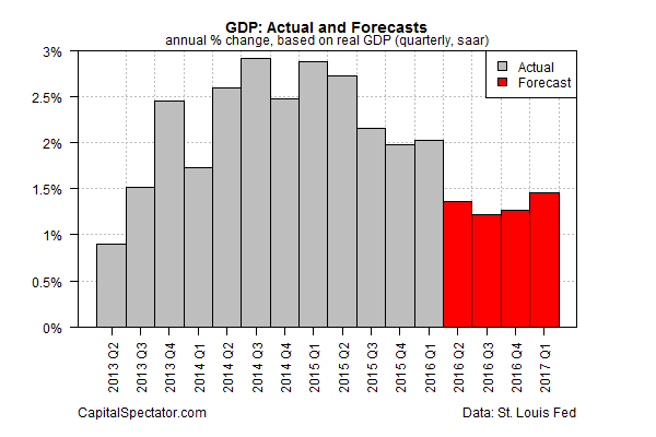
Here’s how the results stack up. The chart below shows the forecasts for year-over-year changes in GDP for the next four quarters, starting with Q2, via the red bars. For perspective, the actual results for recent history are shown by the gray bars, which currently ends with this year’s Q1 data.

The main result is that the outlook calls for a sizable deceleration in year-over-year GDP growth. For Q2, economic output is projected to slow to a roughly 1.4% rise vs. the year-earlier quarter. That’s down from 2.0% in Q1. If the projection is accurate, it marks the weakest year-over-year growth in three years.
The specific numbers for the forecasts probably aren’t reliable. Rather, the key point here is that the model is projecting that the macro trend will ease sharply in Q2. Does the slowdown constitute a recession warning?
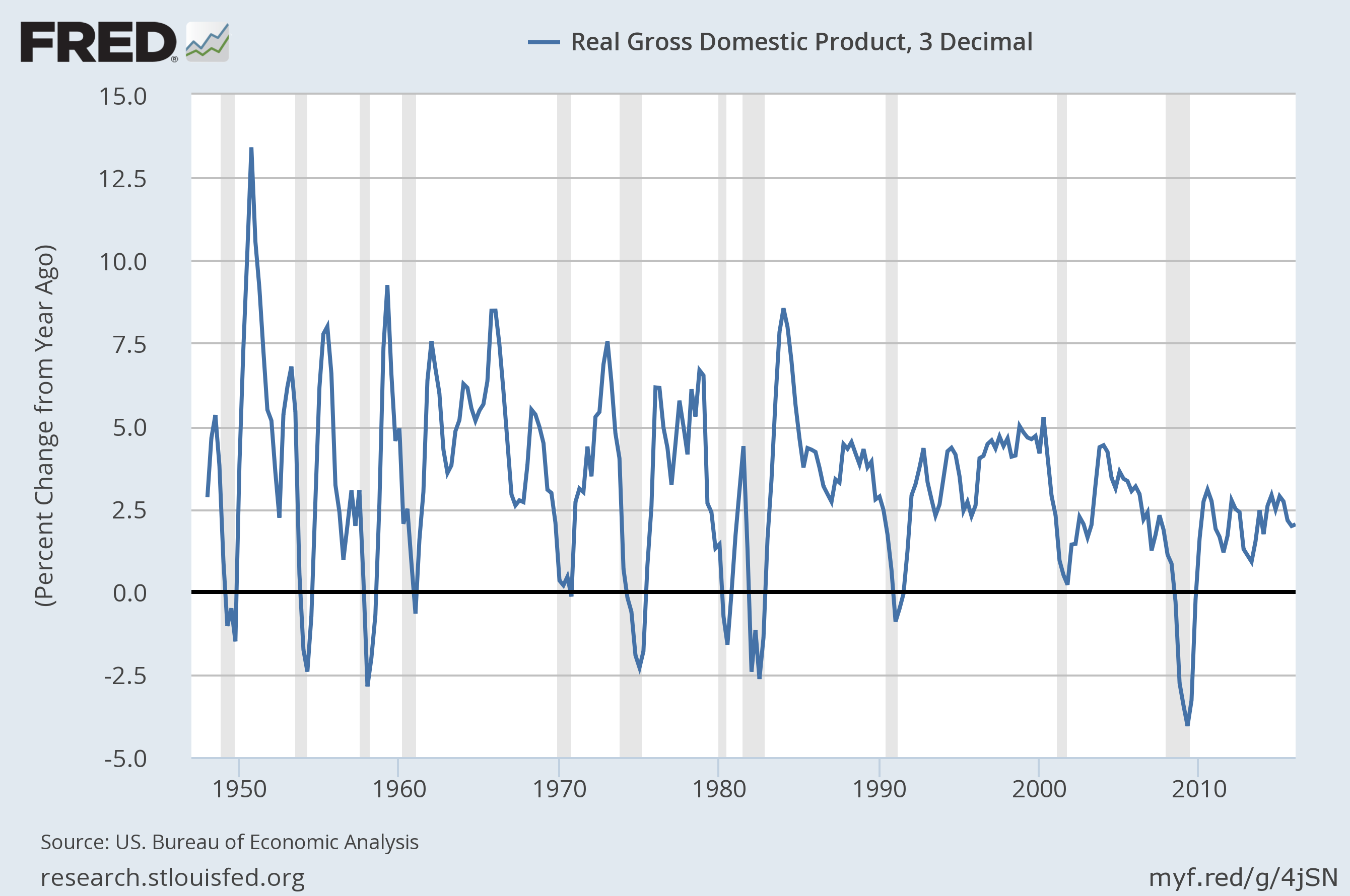
For perspective, we can look at the historical record for year-over-year changes. As the next chart shows, a 1.4% annual rise in GDP is weak, but not necessarily weak enough to mark a smoking gun for a new recession. But it’s not particularly encouraging either, especially in the current climate. For now, let’s label it a gray area.

The question, of course, is whether the forecast is reliable in terms of the directional outlook–down? We’ll soon see. Note that the historical results for the underlying data sets for the model will be updated each time a new GDP report is published. The next update is June 28, when the third Q1 GDP estimate is released. Shortly after, I’ll re-run the numbers and post the revised forecasts.
In the grand scheme of GDP analysis, the outline above is one more forecast in a sea of predictions. I’m cautiously optimistic that the model offers useful context–in broad brush terms–by signaling deceleration in Q2. Let’s see how the actual figures compare when the Bureau of Economic Analysis publishes the “advance” GDP report at the end of July.
