Diversification is famously described as the only free lunch in investing and so it’s no surprise that modeling, analyzing and otherwise dissecting the concept is a core part of portfolio design and management. The correlation coefficient is often the go-to metric in this corner of finance. But like any one statistical measure, there are pros and cons with correlation and so relying on it exclusively can be misleading at times. Fortunately, there are alternatives.
For some perspective, let’s review how these alternatives compare with correlation for a handful of ETFs. Although the following review isn’t comprehensive, it’s a good starting point for diversifying your toolkit of diversification metrics in the pursuit of a deeper, richer profile for investing’s so-called free lunch.
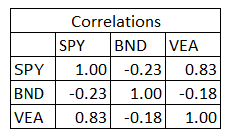
As a baseline, let’s begin with the standard correlation data on three funds, representing US equities, US bonds and foreign stocks in developed markets: SPDR S&P 500 (NYSE:SPY), Vanguard Total Bond Market (NYSE:BND), Vanguard FTSE Developed Markets (NYSE:VEA), respectively. The underlying data: daily returns for the five years through yesterday’s close (May 22).

As you’d expect, the results show a modest negative correlation between stocks and bonds while the correlation between US and foreign equities is relatively high. Recall that correlation values range from 1.0, a perfect positive correlation, to 0.0 (no correlation) to -1.0 (perfect negative correlation).
Cointegration For many applications, a simple correlation profile may suffice. But sometimes it’s prudent to go deeper. One possibility is to consider how the numbers stack up for mean reversion. To quantify the relationship between two time series on this front we can look to cointegration. If the data sets are cointegrated, any deviations in the trend relationship is expected to mean revert. An obvious example: two S&P 500 Index funds will exhibit a high degree of cointegration and so any deviation between the two portfolios will likely be temporary.
To test for cointegration we can use an Augmented Dickey Fuller test. The basic methodology used below is defined by testing for a unit root in the spread between two time series. (For details on implementation using R code, see the analysis here.)
The critical output is the p-value. A “low” p-value is often defined as below 0.05, which indicates a mean-reverting tendency. By contrast, p-values above 0.05 suggest no mean-reverting tendency.
Crunching the numbers for SPY and BND based on prices for the trailing five-year window produces a p-value of 0.23. In other words, SPY and BND don’t exhibit a mean-reverting tendency. That jibes with the correlation data in that SPY and BND tend to move independently of each other.
The p-value for SPY and VEA is even higher at 0.39. The implication: there’s an even weaker case for expecting a mean reversion tendency in US and foreign developed market stocks, at least for the current trailing five-year window. That’s surprising and requires additional research. Intuition implies that US and foreign shares exhibit a higher degree of mean reversion vs. US stocks and US bonds. Yet the p-value data suggests otherwise.
Beta Another way to measure the diversification benefit (or lack thereof) between assets is with beta, a widely used risk measure in financial analysis. This measures how an asset’s volatility compares with a benchmark asset. A beta reading of 1.0 indicates that an asset offers the same level of volatility as the benchmark, which implies that the diversification value is essentially zero. A beta of 1.5 reflects volatility that’s 50% higher than the benchmark; a 0.5 indicates volatility that’s 50% below the benchmark.
Running the numbers on SPY and BND, using BND as the benchmark, produces a -0.94 beta for SPY. That tells us that there’s a deeply inverse relationship between the two assets. By contrast, SPY’s beta is 0.74 with VEA as the benchmark — an indication that SPY’s risk is closely (but not perfectly) aligned with VEA.
R-squared. Yet another way to compare the relationship of assets is with a metric known as R-squared, which is calculated with a regression model. This metric is related to correlation and beta and so the three tend to confirm one another.
R-squared values range from 0 to 100, with 100 showing that all of an asset’s movements are explained by the benchmark asset; 0 indicates the benchmark asset offers no relationship for explaining the target asset’s movements.
The R-squared between SPY and BND for the past five years is a low 0.05, which indicates very little of SPY’s volatility is “explained” by BND. The R-squared for SPY via VEA, by contrast, is relatively high at 0.70.
Standard Deviation Keep in mind that standard deviation (volatility) can also be used to quantify the degree of diversification. As a simple example, consider that SPY’s trailing five-year volatility is roughly 11%. Meantime, vol for the iShares Core Moderate Allocation ETF (AOM) over the same time period is less than 5%. By this comparison, diversifying into a multi-asset class portfolio from US stocks cuts risk by more than half. As such, the value of diversification, one can say, is significant, at least from the perspective of reducing risk.
The main takeaway is that correlation isn’t the only kid on the block for quantifying diversification. Sometimes it’s all you need, and quite often it’s it’s an obvious place to start the analysis. But there are times when a deeper dive is warranted, perhaps because the portfolio design is unusual or the assets are esoteric. In those cases, it’s wise to look beyond correlation.
